Time Travel with Data – Use cases and techniques

Data Historization is a pretty frequent need in data analytics that should be managed at some point in most of the companies. Let’s just think about the following use case. A company is having it’s sales order backlog in it’s ERP system. Management is interested in the backlog, but not only how much it is currently, but how this backlog evolved through time, how it looked like in the system yesterday or a week ago. As this is not a default feature of all ERP systems (or any other applications) to store historical data, this is something we need to take care of. In this current blog post I’ll share some concepts and techniques I usually apply in this topic.

There are many different conditions that matters when choosing the right historization method. It is also possible that in an ecosystem multiple different methods are used. Here I will explain a bit about the 3 techniques I’m using the most.

• Slowly Changing Dimensions Type 2
• Data Snapshot
• Refine from logs

Slowly Changing Dimensions Type 2

Slowly Changing Dimensions or SCD is a typical historization method in data engineering. There are several types defined, but the one I use the most is the Type 2 (https://learn.microsoft.com/en-us/data-engineering/playbook/articles/scd-using-change-data-feed). I think SCD2 is a method that needs relatively small storage, but provides the availability of even each changes of the data. We can define any point in time for that we can get to the effective data.

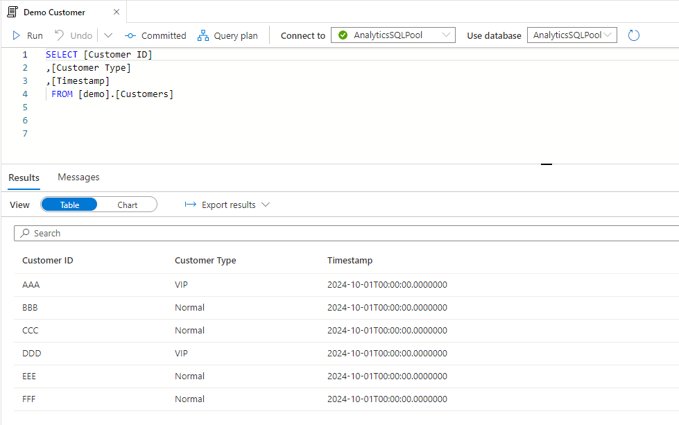
Let say we Customer data that we want to historize. For simplicity we work with three attributes: Customer ID, Customer Type and Timestamp when the record has changes last time:

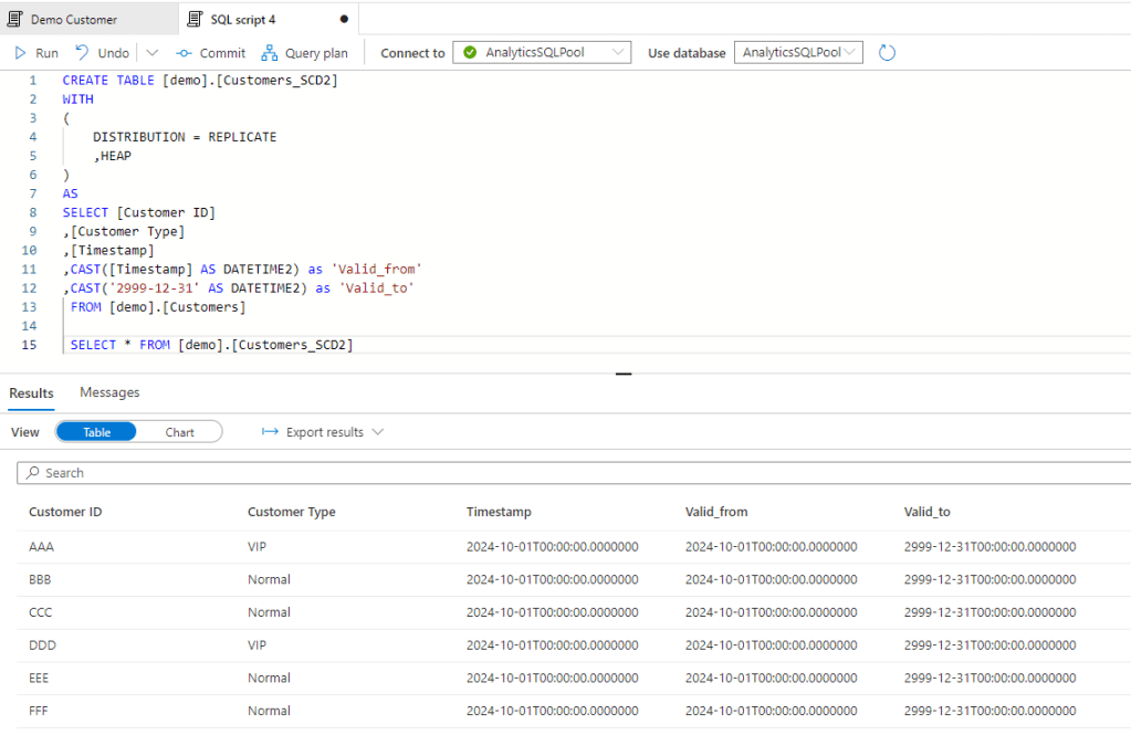
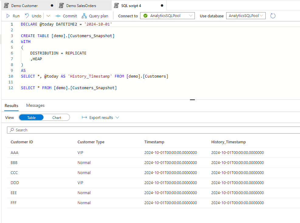
First we should set up the SCD2 history table with an initial full copy.

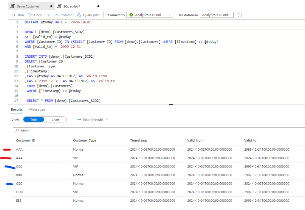
Then we want to track all changes from one day to another – it can be even every hour, but now we will work with daily changes. Let’s two changes for the next day.

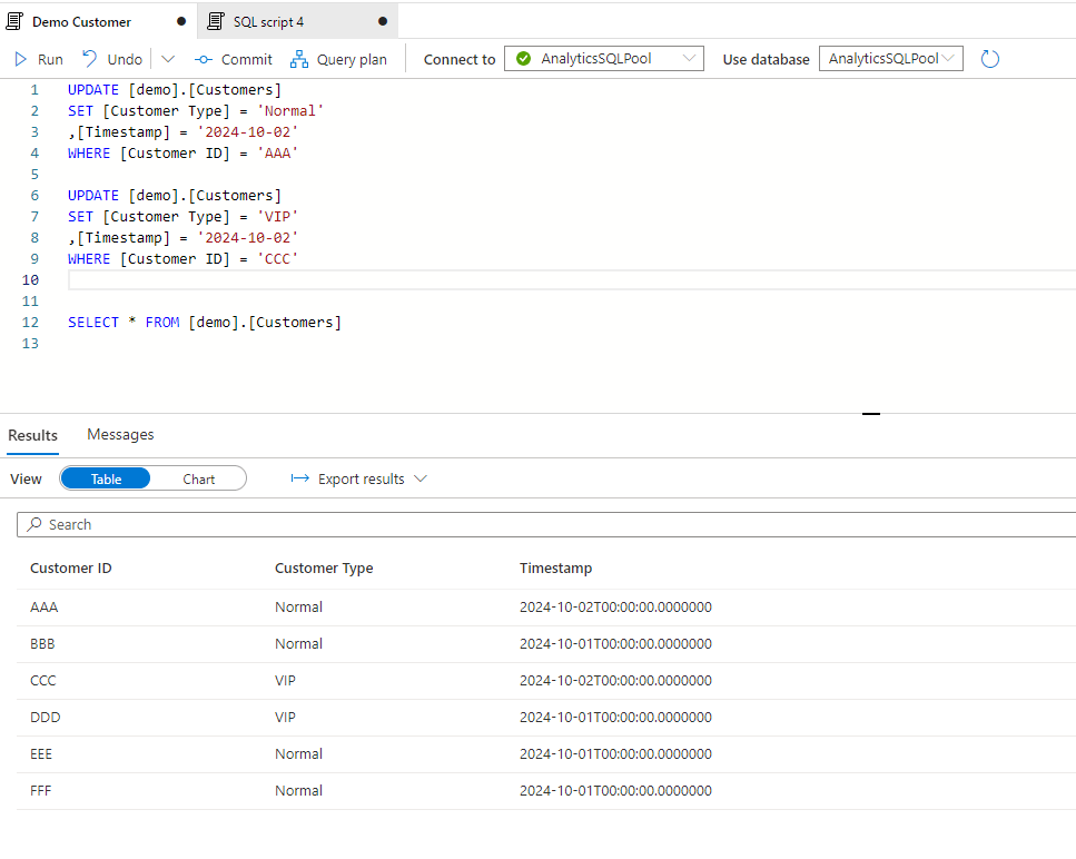
Now let’s run the historization that should create two new records for customer AAA and CCC, and close their current setup with the valid_to field. Note the newly created and historic items for that two customers

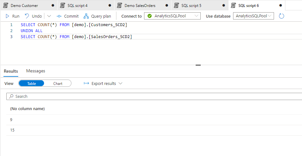
I’ve done some further changes for the following day and also created an SCD2 table for Sales Orders data. The 3 days history now contains the following nr of records for the two tables:

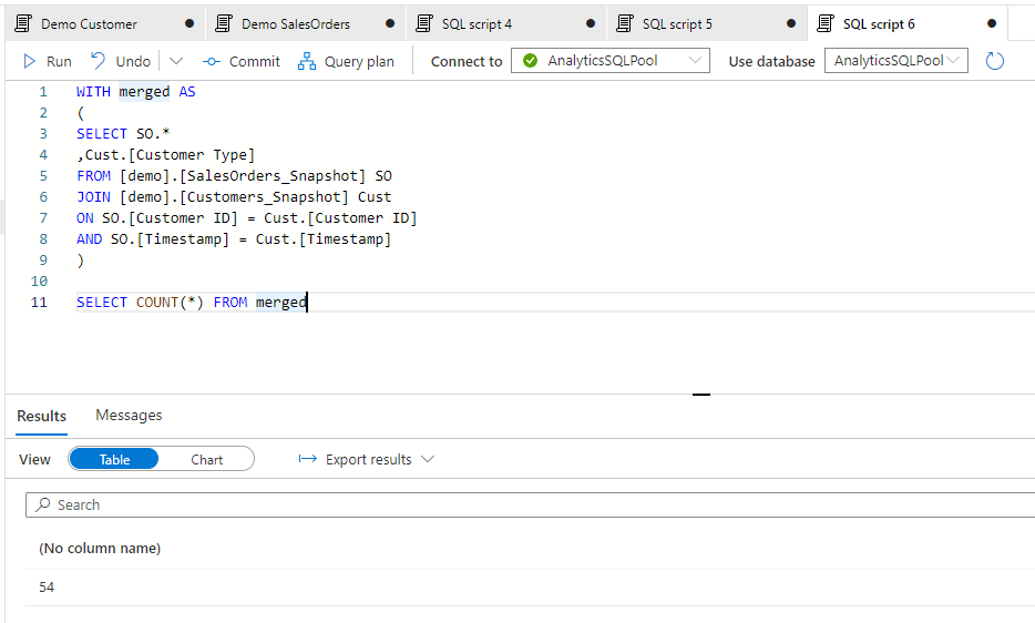
Let’s see now how we can work with it by merging the two, assuming we need to see the daily movement of Quantity by Customer Type. First we should merge the two tables. First if I just merge it by the Customer ID I can see the following:

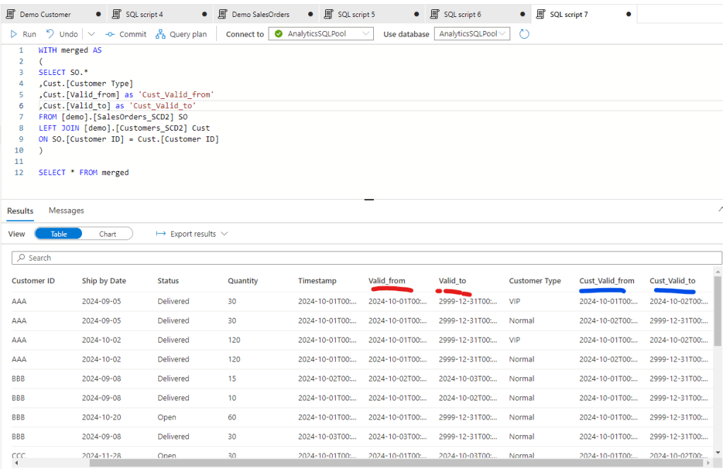
All together we have a query of 23 records and to get the needed data we need to set the WHERE clause both for the SO Valid dates and the Customer Valid Dates.

However this last final calculation is probably done in a BI tool, so this duplicated condition should be defined in each measures we create. Also the Descartes multiplication of the two tables will increase a lot through time so after a longer period the size of the merge tables would be much higher. To avoid that we can consolidate the tables with the original query applying a condition there to merge the tables only if the valid dates are in the same time slot.

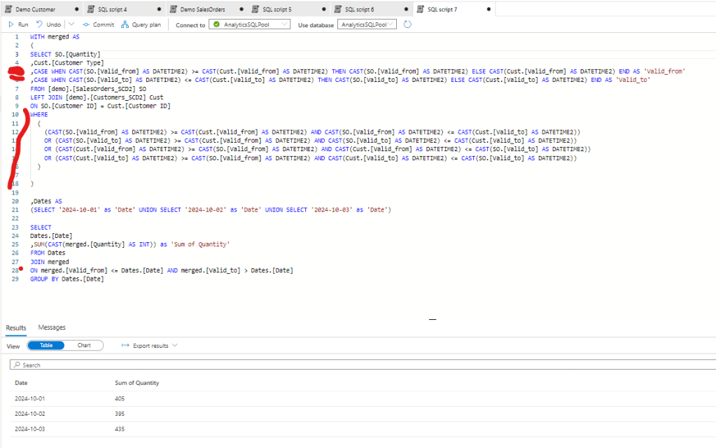
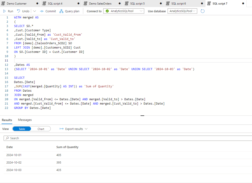
With that we push back the consolidation to the source query and we need to write only one condition in the BI layer. Also the number of records is reduced to 22 that doesn’t seem to be a big decrease for this small table, but if we have millions of rows in our fact tables and thousands of row in our dimension table, and in case we need to merge not only 2 but 4-5 tables, this difference can be significant.

However SCD2 historization has one disadvantage on the BI side. With this structure you won’t be able to create a star schema in your semantic model. As all your measures should define the target date and the measures will evaluate it by tables, you cannot create relationships between your tables as you cannot exactly define the effective dim values at a single point in time.

Data Snapshot

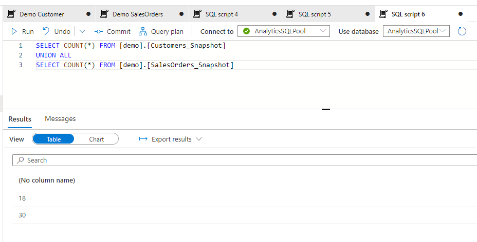
Data Snapshots are much easier to create and work with. All the snapshot is doing is the create a copy of all records each days about their current status. So is we have a tables of 10 records, after 5 days we will have 5 * 10 = 50 records. So we can already see that the drawback of this method will definitely be the size of the tables that’s significantly higher than in the SCD2 method.

Let see how we can generate the snapshots for similar changes of the original table. First let’s create the Snapshot table. Note that we created another History_Timestamp fields that’s showing which day the history was created.

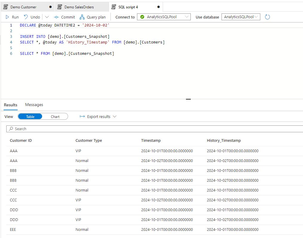
And let’s do some changes again in the Customer table for day 2. After the changes are done let’s create the snapshot for day 2:

After creating and populating the same snapshot table for Sales Orders, the records of the two tables looks like this:

And after merging the tables:

The good thing with this is the ease of join as due to the exact History_Timestamp, we can join the history tables with each others easily. This behavior also enables us to create a surrogate key with the original key and the timestamp and with that we can even create a star schema in our semantic model connecting 2 or more historical tables together.

Definitely the bottleneck here is the storage as the history tables will be huge. This timestamp method is only recommended if we have relativel small dimension tables with few hundred records.

Refine from logs

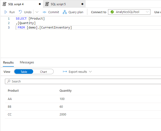
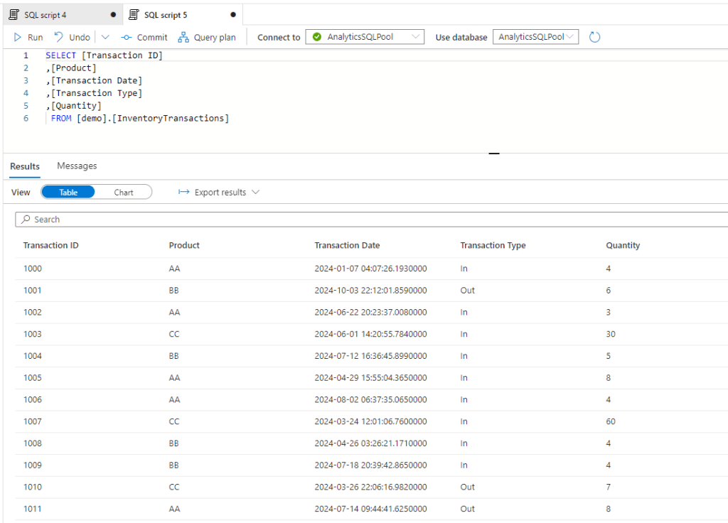
In this example let’s think about a use case of inventories. In ERP systems several times there is a table for current inventories that is showing the level of inventory for items effective now. And there is another tables that details all inventory transactions with their dates and quantities.

Let say we want to see how much the inventory was on ‘2024-03-31’ for the three products. The was how we can approach it is a reverse calculation of transactions against the current state. So whatever has been received to the warehouse should be subtructed and all that’s delivered to customers should be added.

Current Inventory – Sum of intake between 3/31 and today + Sum of deliveries between 3/31 and today

With codes:

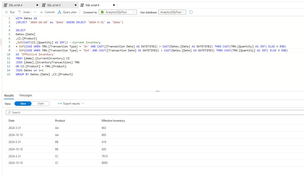
and here we go, we have the historical inventory level on the requested date.

This method is different from the first two methods as it doesn’t require storage capability, so if you don’t have any write access on SQL server or other databases, this method works for you still. However as no phisical data is available, this can be resource intensive on the compute side of your BI tool.

Conversion of methods

This is also possible to convert the different methods to another. Let’s say you have an SCD 2 history table, but you would like to create a model so you want to convert ot to a Snapshot table. This is possible by querying those records by dates which were effective that time. So here is our Customer SCD2 table:

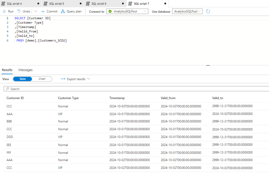
we can query this by the dates:

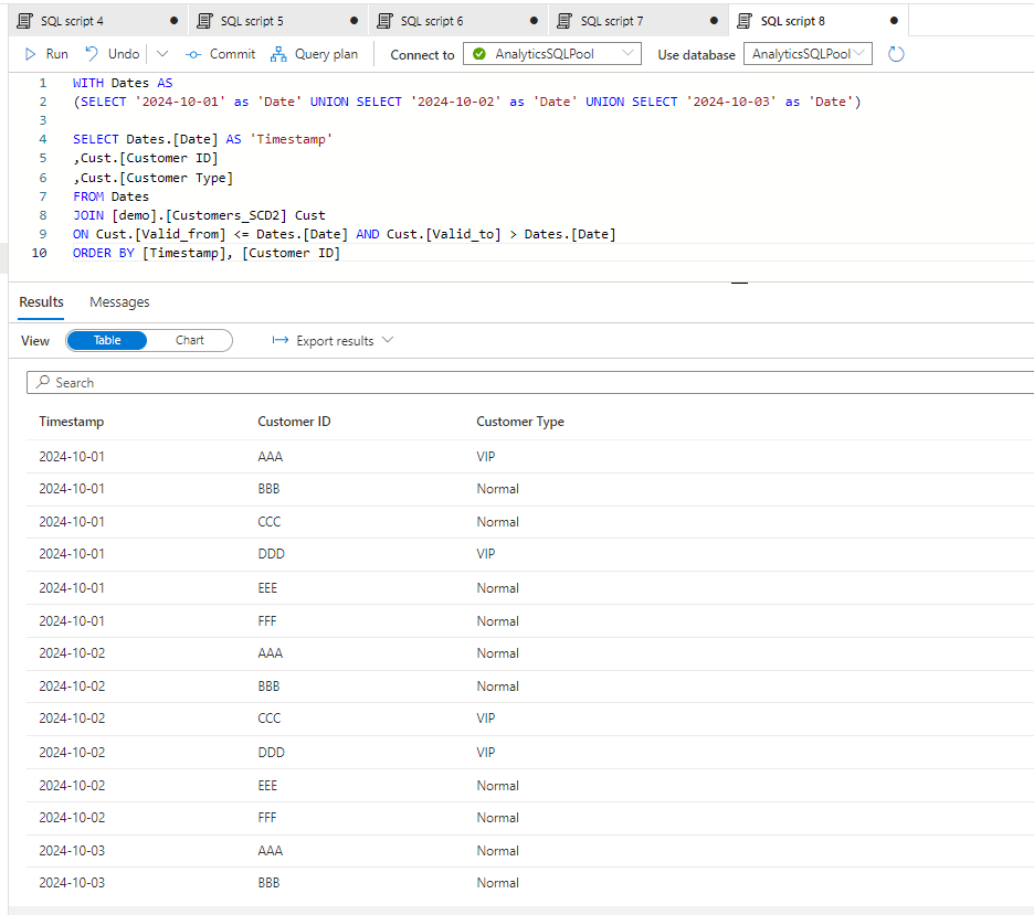
And here we have the Snapshot created from the SCD2 table.

Conclusion

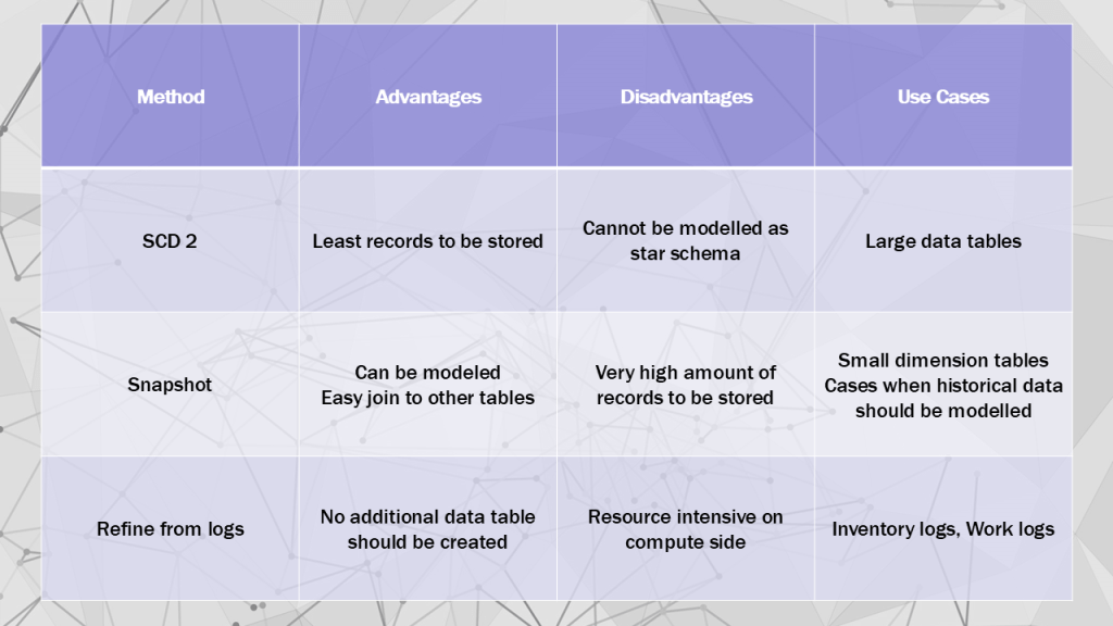
The above methods can all be good for historization, you need to evaluate which one to choose. I think the below matrix is showing well the advantages , disadvantages and use cases for each:

Hope you found it useful.

Cheers!